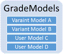
GradeModels
About
Simulation.Model.GradeModels represents a
collection of tree grade classification models. A grade model in OSM predicts
the proportion of stems in a tree record that should be assigned to each grade
class; including class changes (transitions) during simulation. The tree grade
classification system depends on the grade model. OSM can accommodate tree
grade classes ranging from 1 to 255. Depending on the classification used,
grade class could indicate tree form class (e.g., forked top, straight bole) or tree quality class (e.g., amount of rot, defects,
and/or damage) or some combination of form and quality.
Collecting
tree grades in the field and predicting tree grades in OSM can be useful for
simulating short-term and long-term value of alternative stand improvement
prescriptions. When simulating harvest prescriptions in OSM, tree selection can
be directed toward maintenance or improvement of high value trees through Priority and Retention commands.
A
user grade model (specified in a text file with a .grade extension) can specify grade predictions and transitions by
species and DBH class. Alternate models (files) can be built for different
stand or site conditions; each model can be loaded using a single command (LOAD). Variant model developers are free to build more
complex models that predict tree grades using a number of site, stand, and/or
tree properties. Both user and Variant grade models are loaded to the same
collection (GradeModels) so users can easily switch
models with a single command (CURRENT) between stand
simulations.

Variant
grade models:
1)
are
less onerous for users (no grade calibration file needs to be loaded);
2)
ought
to run faster during simulation;
3)
ought to be well tested.
User
grade models can be useful for:
1)
adapting
to a different grade classification system;
2)
testing
alternate grade models;
3)
providing grade predictions in cases where the Variant does not.
Tree grades collected in the field can be specified in the Tree List using the Grade column. Grades ≤ 0 or
null in the Grade column will be predicted using the CURRENT
grade model if ENABLED. Only species that are
represented in the grade model will get grade predictions. Grade predictions
occur when the tree list is loaded and before the first simulation cycle
begins. Grade predictions for recruits and grade transitions for existing trees
occur at the end of a simulation cycle after all tree list changes have been
accepted; therefore, no grade transitions will be apparent in reports until
Cycle 1.
When grade predictions or transitions do occur, they cause
the tree record to be partitioned into new tree record objects; one for each
new class predicted. Number of original tree record stems are also
proportionally distributed to the partitioned records by class according to the
grade model. After partitioning occurs, all tree record properties, other than
number of stems and grade class, stay exactly the same; even Tree ID. This
permits grade transitions to be tracked by tree ID in results if desired.
Unfortunately,
partitioning trees into new grade classes can result in near-exponential growth
of tree records from cycle to cycle and can severely reduce model performance
to the point of memory failure. An elegant solution to this problem is to make
transitions random if the number of tree records exceed a user defined
threshold; see command RandomLimit
for detailed discussion of the value and cost of this feature.
Commands
GradeModels
Enabled TRUE or
FALSE {DEFAULT =
False}
Load {model name} {local file path
*.grade}
Current {model name}
Enabled
If a
Variant defines a grade model, you will need to enable it to get OSM to use it.
By default, grade models are not
enabled because they reduce simulation performance.
SIMULATION.MODEL.GradeModels.Enabled
TRUE
Current
Current
grade model used by OSM. To switch grade models, use:
SIMULATION.MODEL.GradeModels.Current
Name
Name: model ID (name) in the
collection of GradeModels. Double quotes are required
around the name if it contains spaces.
This
command is provided to permit users to switch back to the Variant grade model
after loading a user grade model during the same session. Also, the Variant may
declare multiple grade model versions for users. This property allows a user to
switch to a different model between stand simulations. Consult Variant
documentation for declared grade models, if any. This functionality is also
exposed in the API.
Load
To
load a user-defined grade model use:
SIMULATION.MODEL.GradeModels.Load
Name “C:\...\TextFile.grade”
Required
arguments:
1)
Name: used to ID the model in the
collection of GradeModels. Double quotes are required
around the name if it contains spaces.
2)
File: local absolute or relative
file path to the user-defined grade model; relative to command file. Double
quotes are required around the path if it contains spaces.
When
LOAD is called:
1)
OSM
attempts to read and build the user-defined grade model.
2)
OSM
stores the model in memory in GradeModels for the
remainder of the session.
3)
ENABLED
is switched to TRUE, if not already true.
4)
CURRENT
is set to the user-defined model name, which instructs OSM to use the
user-defined grade model.
Important:
·
If
you load a new grade model with the same name as an existing grade model
(Variant or User), the existing grade model will be replaced with the loaded
version. It is therefore wise to consult Variant documentation on grade model
names to avoid using.
RandomLimit
Adjusts
the number of tree records required before grade transitions become random
events; e.g.,
SIMULATION.MODEL.GradeModels.RandomLimit
1000
Required
arguments:
1.
Limit: number of tree records required
before grade transitions operate as random events.
·
Default
= 1000
·
Minimum
= 0; transitions always occur as random events.
·
Maximum
= 2,147,483,647; transitions never occur as random events.
As
discussed earlier, partitioning tree records into new grade classes each cycle
can exponentially reduce simulation performance to the point of failure.
Assuming only 10 initial tree records and 10 new ingrowth records per cycle, a
grade model with 3, 4, and 5 grade classes could potentially cause the number
of tree records to balloon to 52 million, 192 billion, and 69 trillion records
after only 20 cycles.
A
partial solution to this problem is to make class transitions operate as random
events, where probability of transitioning to one or more classes is equal to
the annual or periodic transfer proportion of the class. If that probability is
greater than a random number between 0 and 1, the entire tree is transitioned
to other classes in proportion to the respective transfer ratios provided for
those destinations. However, if initial tree records are few, random
transitions can lead to very erratic grade transitions over time. A final
solution to this problem is to only enable random transitions if the number of
tree records is greater than some limit.
By
default this random transition limit is set to 1000 records. Again, assuming
only 10 initial tree records, 10 new ingrowth records per cycle, and assuming a
transfer probability of 5% per 5-year cycle, a grade model with 3, 4, and 5
grade classes with a random limit = 1000 would cause the number of tree records
to expand to approximately 7, 39, and 47 thousand records after 20 cycles.
Reducing the random limit to 100 would reduce these estimates by more than
half. Despite this solution, given the negative impact of increasing the number
of grade classes on simulation performance, the grading system should use as
few classes as possible (2-3 preferred; >5 strongly discouraged).
Example
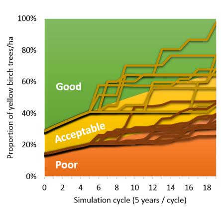
effects of Random Limit on simulation results is presented below for six
initial yellow birch tree records in a mixedwood stand in New Brunswick. In
this example, three grades (poor, acceptable, and good) are predicted at cycle
0 and then transitioned for twenty 5-year cycles (100 years) using:
·
Good
à Acceptable @ 0.5% per year
·
Good
à Poor @ 0.25% per year
·
Acceptable
à Poor @ 0.5% per year
The
stacked area fill in the background of the figure below shows the proportion of
grades over time resulting with random limit set to one million, which
effectively turns random transitions off, compared to ten scenarios (stacked
lines) with random limit set to 1000 (default). Note results for all eleven
simulations are identical up to cycle four. In cycle five, number of tree
records exceed 1000, which causes random transitions to occur at the end of
cycle five. For all yellow birch trees, the average proportion of poor and
acceptable grades for the ten stochastic simulations was within 1% point of the
deterministic simulation at 100 years. The deterministic simulation resulted in
20 times more records by year 100 and was 7-8 times slower to execute compared
to the average stochastic run.

Ability
to make grade transitions deterministic or stochastic can be useful for
simulating the probability of achieving certain prescription targets over the
long-term. It may be that a harvest prescription appears attractive under a
deterministic simulation, but 4 times out of 10 stochastic simulations the
treatment fails to deliver an adequate supply of high value trees for
subsequent entries.
Defining a user
grade model
A
custom grade model is defined in a text file (*.grade) and loaded (LOAD) to OSM before stands are simulated. This model
specifies Predictions and Transitions of grades by Variant Species and by 1 cm DBH classes.
General
arrangement of keywords (bold) and arguments in the text file is shown in the
example below; general descriptions (gray) are omitted in text file.
|
Species SM RM YB BE RO |
Species Filter |
|||||
|
|
|
|
Grades |
Total Check |
||
|
|
Predictions 1 2 3 |
DBH* |
1 (Poor) |
2 (Acceptable) |
3 (Good) |
|
|
|
|
5 |
14.48 |
9.86 |
75.66 |
100.0 |
|
|
|
10 |
14.07 |
12.45 |
73.48 |
100.0 |
|
|
|
20 |
14.23 |
16.17 |
69.60 |
100.0 |
|
|
|
30 |
15.69 |
17.97 |
66.34 |
100.0 |
|
|
|
40 |
18.46 |
17.84 |
63.69 |
100.0 |
|
|
|
50 |
22.54 |
20.46 |
57.00 |
100.0 |
|
|
|
70 |
34.61 |
22.39 |
43.00 |
100.0 |
|
|
|
|
|
|
|
|
|
|
Transitions 1 |
|
Annual proportion of class 1 -> 1 2 3 |
|
||
|
|
|
0 |
100.00 |
0.00 |
0.00 |
100.0 |
|
|
|
5 |
99.25 |
0.50 |
0.25 |
100.0 |
|
|
|
|
|
|
|
|
|
|
Transitions 2 |
|
Annual proportion of class 2 -> 1 2 3 |
|
||
|
|
|
0 |
0.00 |
100.00 |
0.00 |
100.0 |
|
|
|
5 |
0.00 |
99.50 |
0.50 |
100.0 |
|
|
|
|
|
|
|
|
|
|
Transitions 3 |
|
Annual proportion of class 3 -> 1 2 3 |
|
||
|
|
|
0 |
100.00 |
0.00 |
0.00 |
100.0 |
|
*DBH in 1 centimeter classes only; inches not supported. |
||||||
Actual
text in the file for the above model is shown below (comments in green).
#Example Tree Grade Classification Predictions & Transitions
# 1 = Poor; 2 = Acceptable; 3 = Good
# Limited to shade-tolerant hardwood
Species SM RM YB BE RO
Predictions 1 2 3
5 14.48 9.86 75.66
10 14.07 12.45 73.48
20 14.23 16.17 69.60
30 15.69 17.97 66.34
40 18.46 17.84 63.69
50 22.54 20.46
57.00
70 34.61 22.39
43.00
Transitions 1
0 100.00 0.00 0.00
Transitions 2
0 0.00 100.00 0.00
5 0.50 99.50 0.00
Transitions 3
0 0.00 0.00 100.00
5 0.25 0.50 99.25
Species
Different
grade models for different species or species groups can be defined in the same
text file; one after another. The keyword Species
declares a new grade model for a species or species group. Predictions must be declared and Transitions can be optionally declared below each Species keyword.
Species A B C
Predictions…
Transitions…
Species D E F G
Predictions…
Transitions…
Variant
keys, USDA plant or genus codes, and species
groups previously declared can be used to assign predictions and
transitions to specific species. If no species codes are listed after Species, then the grade model is
assigned to all species. Subsequent Species
models will overwrite previous Species
models where individual species overlap.
Predictions
Predictions declare the grade classes in
the model (e.g., 1 – Poor, 2 – Acceptable, 3 - Good) immediately following the
Predictions statement. Classes can be any whole number between 1 and 255. Below
the Predictions statement, grade
proportions (respective of the order classes declared in Predictions) are
listed in rows by DBH class (1 cm). DBH class can be any whole number between 0
and 100. Linear interpolation is used to calculate proportions for any DBH
class not provided. If DBH classes provided do not include 0 or 100, then the
closest DBH class proportions will be used (i.e., no extrapolation). To
maximize simulation performance, OSM pre-calculates predicted grade proportions
by 1 cm DBH class from 0 to 100 cm; therefore, a tree with DBH of 5.6 cm would
use proportions calculated for a 6 cm tree.
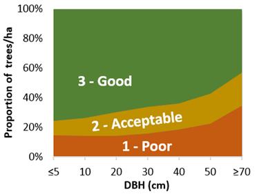
The
following predictions:
Predictions 1 2 3
5 14.48 9.86 75.66
10 14.07 12.45 73.48
20 14.23 16.17 69.60
30 15.69 17.97 66.34
40 18.46 17.84 63.69
50 22.54 20.46
57.00
70 34.61 22.39
43.00
, would
result in the following proportions of grades assigned to all trees by 1 cm DBH
class.

These
predictions will occur for all tree records where Grade is null or 0, which
include initial tree records in cycle 0 and ingrowth in cycles
≥1.
Transitions
Transitions
declare the annual proportion(s) of one class that is predicted to
transfer to another class(s). If no transitions are specified, no transitions
occur. Transitions do not need to be declared for every grade class; but when
declared for a class, the class must have Predictions
(i.e., the class must be listed after Predictions).
The
single class stated immediately after Transitions defines the transfer source, while
the proportions listed following the DBH class (much the same as Predictions)
under Transitions tell OSM how much of the source class to transfer to the
destination classes annually. As with Predictions, linear interpolation is used
to calculate proportions for missing DBH classes, no extrapolation occurs, and
transition proportions by 1 cm DBH class from 0 to 100 cm are pre-calculated by
OSM.
The
following transition model (from above):
Transitions 1
0 100.00 0.00 0.00
Transitions
2
0 0.00 100.00 0.00
5 0.50 99.50 0.00
Transitions 3
0 0.00 0.00 100.00
5 0.25 0.50 99.25
,
would yield the following behaviour:
·
Class
1 (poor) would transition to itself.
·
Class
2 (acceptable) would
o For DBH = 0 cm, transition
back to itself.
o For DBH ≥ 5 cm,
transition at a rate of 0.5% / year to class 1 (poor).
o For DBH > 0 and < 5 cm,
transition at a linearly interpolated annual proportion to class 1.
·
Class
2 (good) would behave much the same as Class 2 except that a maximum of 0.25%
and 0.5% will be annually transferred to class 1 (poor) and 2 (acceptable),
respectively.
Because
class 1 in the example above always transitions back to itself at 100% the
transition declaration for class 1 should be left out of the text file to
improve performance; OSM will not need to query the transition for class 1 at
all if it does not exist.
When
years per simulation cycle are > 1, the annual transition proportion of the
source class is converted by OSM to a periodic proportion using the compound
interest formula. The relative proportion transferred to other classes is
multiplied against the periodic proportion to yield final periodic transfer
proportions. For example:
|
Class 3 -> |
1 |
2 |
3 |
|
Annual |
0.250% |
0.500% |
99.250% |
|
Periodic (5 year) |
1.231% |
2.463% |
96.306% |
Note
that annual and periodic simulations will not yield exactly the same results
because under annual cycles, transitions in year one may cause different
transitions to occur in year two; e.g., a tree can transition from class 1
-> 2 -> 3 within a 5-year period using annual cycles; whereas, under
periodic cycles a tree can only undergo a single source -> destination
transition. At the end of a 50-year simulation using a random test stand, the
transition model example above resulted in <0.4% difference in absolute
class proportions using annual cycles compared to 5-year cycles. Some of this
difference could be attributed to slight differences in tree growth and
mortality under annual vs. periodic simulations, due again to more integrated
model behaviour under annual cycles. Despite minor difference in model results
between annual and periodic cycles, as a general rule, it is recommended that
years per simulation cycle closely match years per measurement in permanent
sample plots used to calibrate models.